In document image processing pipelines (including OCR and music OCR), accounting for the rotation of the document, which is often introduced when scanning images, can dramatically improve the accuracy of subsequent image processing stages. Consider the following score of Bach’s Invention #1 (BWV 772) that has been obtained from the Mutopia project and rotated exactly 2 degrees clockwise:
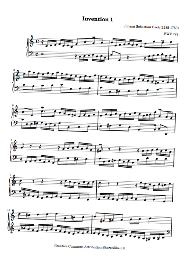
In a music OCR pipeline, undoing that rotation before trying to detect staff lines, clefs, and other symbols in the score can lead to significant improvements in recognition accuracy. This could be done in a brute-force manner by trying various angles of rotation (0.5°, -0.5°, 1.0°, -1.0°, and so on), rotating the document, and checking if the ratio of black pixels per line increases. If it does, it’s probably because the staff lines are better aligned with the x axis of the image. While this may work, it’s both fragile and computationally-expensive.
A more principled solution to this problem would be to use the Hough transform to fit lines through the edges in the image. In case of music scores, we’d end up with lines corresponding to the staff lines, beams, and so on. Since these lines are usually horizontally-oriented, the angle ⍺ between them and the image’s x axis could be interpreted as an estimate of the document’s overall rotation. To undo the rotation, we could then simply rotate the image by -⍺! The advantage of this approach is we only have to rotate the image once instead of brute-forcing our way through possibly hundreds of angles of rotation.
Getting Started
To get started, we’ll have to load our image and detect features through which we should fit lines. For our problem, detecting edges is a good start, and a simple edge detector such as the Canny edge detector will suffice. It simply computes the gradients of pixels in the horizontal and vertical directions and can be efficiently implemented as a 3x3 filter.
Horizontal edges
      [ -1, 0, 1 ]
G_h = [ -2, 0, 2 ]
      [ -1, 0, 1 ]
Vertical edges
      [ -1, -2, -1 ]
G_v = [  0,  0,  0 ]
      [  1,  2,  1 ]
To compute the overall gradient, we simply compute the magnitude of a vector containing the horizontal and vertical components:
G[y, x] = sqrt(G_v[y, x]^2 + G_h[y, x]^2)Luckily for us, Apple’s Core Image framework already implements a CIEdges filter that does just this, so we don’t even have to implement it ourselves.
First, we’ll load the original image of the first page of Bach’s Invention #1:
let invention1URL = Bundle.main.urlForImageResource("bach-invention-01-a4.png")!
let invention1 = CIImage(contentsOf: invention1URL)!
Since it’s easier to work with a grayscale image when computing edges, we’ll convert the image to grayscale with a tonal filter:
let monochromeFilter = CIFilter(name: "CIPhotoEffectTonal")!
monochromeFilter.setValue(invention1, forKey: kCIInputImageKey)
Even though most music scores happen to be grayscale already, there may be subtle variations in color due to anti-aliasing. You may also be working with a scanned image containing annotations written with a colored pen. In any case, explicitly converting the image to grayscale doesn’t hurt.
Now that we have a grayscale image, we can run the edges filter:
let edgesFilter = CIFilter(name: "CIEdges")!
edgesFilter.setValue(monochromeFilter.outputImage!, forKey: kCIInputImageKey)
let outputImageUncropped = edgesFilter.outputImage!
If we set a breakpoint now and preview outputImageUncropped with Quick Look, you’ll find the image contains a white border along the far bottom and far right edges. This occurs because the edge filter is running off the edges of the image (by 1 pixel since we have a 3x3 pixel filter). Since we don’t want these white lines to be picked up by the Hough transform, it’s easiest to just crop the image by 1 pixel around the edges:
let outputImage = outputImageUncropped.cropping(to: CGRect(x: 1, y: 1, width: invention1.extent.width-2, height: invention1.extent.height-2))The result looks like this:
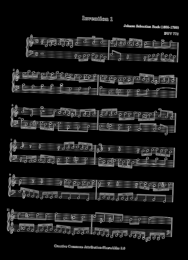
We’ll also convert the resulting CIImage to a NSBitmapImageRep so it’s a bit easier to work with the underlying pixel data:
let imageRep = NSBitmapImageRep(ciImage: outputImage)Please note that NSBitmapImageRep only exists on macOS. If you’re following this on iOS, it’s probably easiest to turn the CIImage into a CGImage and then ask for its underlying data with CGImageCopyData. Since that’s outside the scope of this article and has already been written about extensively, I’ll skip the details here.
Lastly, we’ll threshold the image such that only gradients with magnitude greater than 50% (or 127 in [0-256) RGB values) are considered. Unfortunately, Core Image doesn’t provide an easy way of thresholding images, so we’ll implement this ourselves:
var edgeMap = Array<Bool>(repeating: false, count: imageRep.pixelsHigh * imageRep.pixelsWide)

for y in 0..<imageRep.pixelsHigh {
    for x in 0..<imageRep.pixelsWide {
        var buffer = Array<Int>(repeating: 0, count: 4 /* RGBA */)
        imageRep.getPixel(&buffer, atX: x, y: y)

        edgeMap[y * imageRep.pixelsWide + x] = buffer[0] > 127
    }
}
Here, we simply run through every pixel in the output image and extract its RGBA components. Since the RGB data is the same for each channel in a grayscale image, we simply look at the red (or 0th) component and check if its value is greater than 127. If it is, we set the value in the edge map to true. Now we have all we need to compute the Hough transform and find significant horizontally-oriented lines in the image.
Hough Transform Theory
We know a line can be parameterized as: y = ax + b, where x and y are the parameters and a and b are fixed constants. If two points {x1, y1} and {x2, y2} are on the same line, they will share values of a and b such that y1 = a * x1 + b and y2 = a * x2 + b.
More generally, a set of points P can be said to lie on the same line if, for some fixed values a and b, y = ax + b holds for all points in P. If we could find all unique pairs of a and b, we’d find all the lines in the image. That is the essence of the Hough transform, which, as the name implies, transforms points from x-y to a-b space.
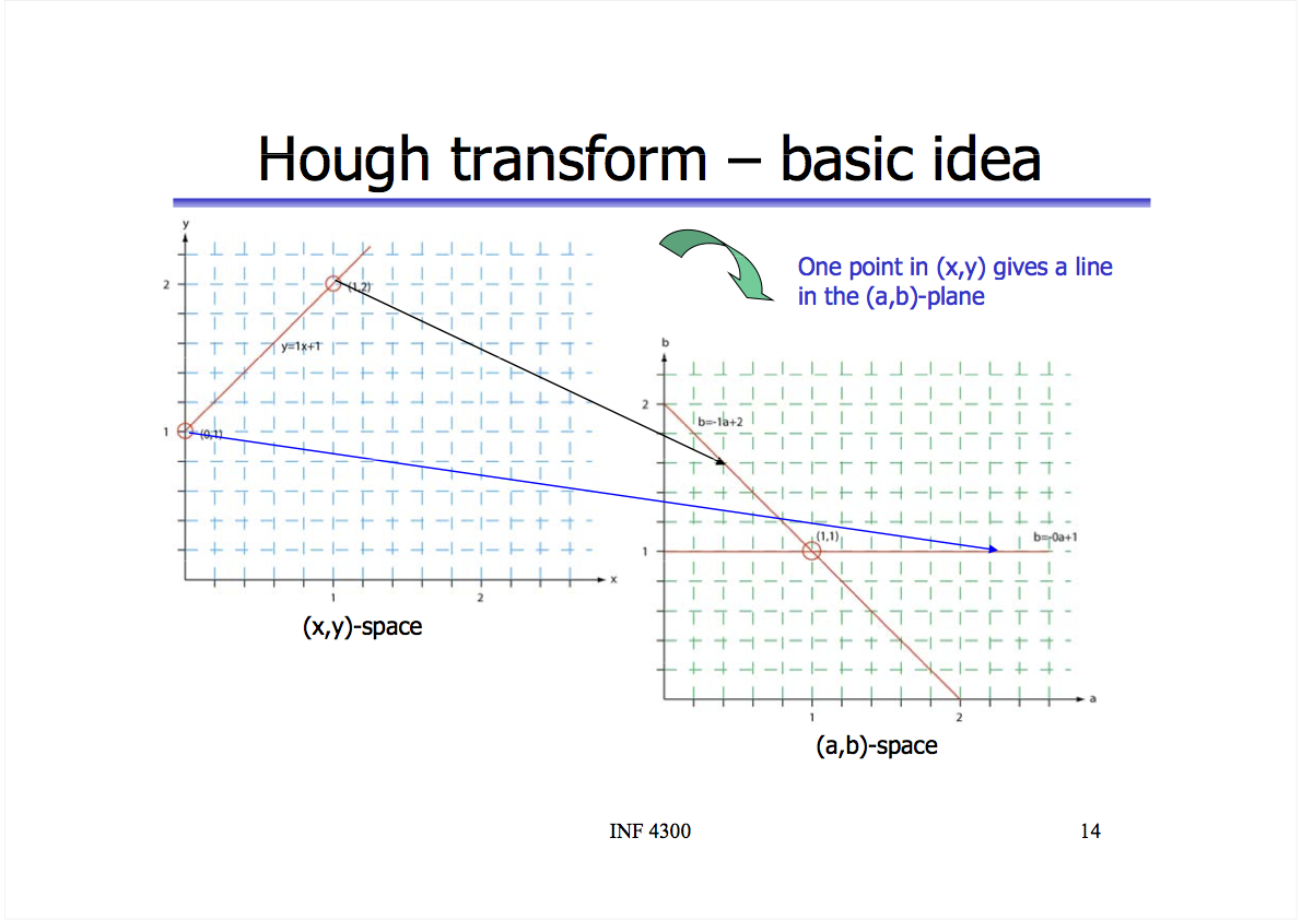
Visually, this slide from the University of Oslo shows how two collinear points in x-y space map to the same value of a and b in a-b space. If there was a third point on the line in the original image in x-y space, there would be a third line intersecting {1,1} in a-b space. The more intersecting lines we have, the more confident we can be there is actually a line for some values of a and b.
In a-b space, a and b are the parameters and x and y are fixed constants. Mathematically, we can get there by simply subtracting ax from both sides of the line equation:
y = ax + b
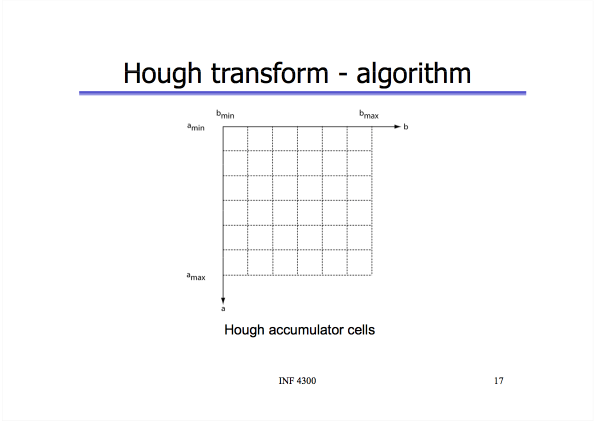
y - ax = bNow to find the actual lines (pairs of a and b), we run through every point {x, y} in the image and every possible value for a and find the value of b using: b = y - ax. We can use a 2D grid of cells (called an “accumulator” in computer vision literature) to count how many hits we get for a given a-b pair. Again, the more hits we have, the more intersecting lines there are in a-b space, the greater the chance of a line in x-y space.
If we sort these cells in descending order by the number of hits and take the top 5, we’d find the lines they correspond to are probably the five longest staff lines in the musical score.
There’s one problem, though. The coefficient a can span an infinite number of values and is impossible to discretize into a grid spanning a-b. Instead, we’ll have to use the polar representation of lines:
x cos(θ) + y sin(θ) = ⍴So, instead of a and b, our fixed constants are ⍴ and θ. In most literature on the Hough transform, θ ranges from -90° to 90°. I find those values really extreme for accounting for tilt in documents, so we’ll use -45° to 45° (most misalignments will probably be on the order of 1-10°). ⍴, the radius, can range from 0 to sqrt(W^2 + H^2), where W and H are the width and height of the image. This is actually possible to discretize on a grid. Everything else still holds for the ⍴-θ space: lines for two points in ⍴-θ space will intersect if the points are collinear in x-y space.
If you’re a little confused, this video by Thales Körting may help clear things up:
Now we’re ready to translate this to Swift.
Hough Transform Implementation
We said that θ will range from -45° to 45°. It’s useful to consider half angles as well, so we’ll loop through angles at intervals of 0.5°: -45°, -44.5°, -44°, … , 44.5°, 45°. If we count 0, that’s (45 * 2) * 2 + 1 points.
let thetaSubdivisions = 2
let thetaMax = 45
let thetaMin = -thetaMax
let thetaCells = thetaMax * thetaSubdivisions * 2 /* plus/minus */ + 1
The radius will range from 0 to sqrt(W^2 + H^2). We’ll also down-sample the radius by a factor of 4, so 4 adjacent pixels will get mapped to the same cell. This helps us deal with lines that may be greater than 1 pixel in thickness, differences in antialiasing, and so on.
let rFactor = 4
let rMax = Int(sqrt(pow(Double(imageRep.pixelsWide), 2) + pow(Double(imageRep.pixelsHigh), 2)))
let rCells = rMax / rFactor
Now we can create a grid of cells (essentially a 2D frequency table) and loop through every pixel in the image that we found to be a significant edge (whose edgeMap entry is true):
var cells = [Int](repeating: 0, count: thetaCells * rCells)

for y in 0..<imageRep.pixelsHigh {
    for x in 0..<imageRep.pixelsWide {
        guard edgeMap[y * imageRep.pixelsWide + x] else {
            continue
        }
For each pixel and each value of θ, we’ll use the polar line equation to compute ⍴. If it lies within bounds, we’ll increment the count of the corresponding cell:
        for theta in stride(from: Double(thetaMin), through: Double(thetaMax), by: 0.5) {
            // r = x * cos(theta) + y * sin(theta)
            let r = Int(cos(theta * M_PI / 180.0) * Double(x) + sin(theta * M_PI / 180.0) * Double(y))

            if r < rMax && r >= 0 {
                let thetaIndex = Int(round(theta * Double(thetaSubdivisions))) + thetaMax * thetaSubdivisions
                cells[thetaIndex * rCells + r / rFactor] += 1
            }
        }
    }
}
After this code executes, the cells containing the greatest counts correspond to the points with the greatest number of intersections in ⍴-θ space. We can now sort them in descending order, consider the top 5, and compute the average θ value:
typealias Cell = (frequency: Int, theta: Double)

var cellTuples = [Cell]()
for theta in 0..<thetaCells {
    for r in 0..<rCells {
        let frequency = cells[theta * rCells + r]
        let thetaScaled = Double(theta) / Double(thetaSubdivisions) - Double(thetaMax)
        cellTuples.append(Cell(frequency: frequency, theta: thetaScaled))
    }
}

cellTuples.sort { return $0.frequency > $1.frequency }
let top5 = cellTuples.prefix(upTo: 5)
let sum = top5.reduce(0.0) { $0 + $1.theta }
let average = sum / Double(top5.count)
If we print the value of average, you’ll notice it’s exactly 2!
To undo the rotation, we can simply rotate the image by -2° and use the newly-rotated image in subsequent image processing operations. You may find the Accelerate framework useful in performing fast image rotations.
While we focused on aligning music scores and had horizontal staff lines to help us out, this could be easily extended to text OCR. Since characters of text are baseline-aligned, we can use the Hough transform to compute the collinearity of the bottom sides of characters.
The full source code for this article can be obtained here.